Hypothesis Testing Series - An End to End Guide to Bayesian Hypothesis Tests - Part 3

 

Hypothesis Testing Series - An End to End Guide to Bayesian Hypothesis Test - Part 3

As the name suggests, Bayesian Hypothesis test is based on Bayes’ Theorm. We start with a prior belief about the population under null and alternate hypothesis. We then use Bayes’ theorem to compute he posterier probability which is basically computing the likelishoood of null and alternate hypothesis after considering the data. Sounds complicated ? Ok let’s break it down in this article and try to understand each step involved along with python code.

Please go through first two articles on the related topic for complete understanding:

An End to End Guide to Permutation Tests | Hypothesis Testing Series #2

Permutation test is one of the most popular non-parametric hypothesis tests. In this article, we will go through the…

indiequant.medium.com

End to End Guide to Hypothesis Testing in Statistics: Concepts, Methods, and Examples

Some experiments, such as testing efficacy of a drug or if a new feature in an app had an impact on app downloads…

indiequant.medium.com

Introduction

Extending to the brief above, in traditional hypothesis testing, we test the null hypothesis using frequentist approach and use a p-value. However, in case of Bayesian hypothesis testing — we update prior knowledge about parameter before observing data and after observing the data.

For this we compute: posterior probability for both null and alternate hypothesis. We can utilize Bayes’ Theorem to compute posterier probability, which updates the probability of a hypothesis H given the observed data D:

posterior probability -> P(H|D)=P(DH)/P(D)=(P(D|H)*P(H))/P(D)

• P(H|D) = posterior probability of the hypothesis H conditional on D,
• P(D|H) = likelihood of data conditional on hypothesis H
• P(H) = prior probability of the hypothesis H,
• P(D) is the marginal likelihood of data.

We can compute this probability for both null and alternate hypothesis and select the one which gives us maximum value.

Problem Statement

Let us try to understand this with the help of an example. Lets say we are testing if a coin is biased or not. Null and alternate hypothesis could be defined in below ways:

• Null — H0​: p=0.5 (probability of heads in case of a fair coin)
• Alternate — H1​: p ≠ 0.5 (probability of heads in case of a biased coin)

We tossed the coin 10 times and got 7 heads. Let's see how we can perform the Bayesian test in Python step by step in this problem.

Code & Explanation

Before we start with implementation, I would like to mention that in addition to definition of null and alternate hypothesis we also need to model likelihood of getting a certain number of heads. That is achieved by a binomial distribution. This would help us computing likelihood of data conditional on null and alternate hypothesis.

import numpy as np
import matplotlib.pyplot as plt
from scipy.stats import binom

# Step 1: 
# We intially assume equal probability of coin being fair or biased since
# we have not seen the data yet i.e. probability of null or alternate 
# being true is equal.
prior_h0 = 0.5 # Prior probability that the coin is fair
prior_h1 = 0.5 # Prior probability that the coin is biased

# Step 2: As explained - below is what we observe 7 heads in 10 flips (data D)
observed_heads = 7
total_flips = 10

# Now lets compute the likelihood of null hypothesis conditional on 
# this is where discussion related to binomial distribution mentioned above is
# helpful
likelihood_h0 = binom.pmf(observed_heads, total_flips, 0.5)

# computing likelihood of alternate hypothesis is slightly tricky. 
# here we assume that probaiblity of heads could be anything between 0 and 1.
# but not .5 (why?)
# we compute the mean likelihood given alternate hypothesis is true by 
# computing the probability mass function value over the range p and taking
# mean of that
p_values = np.linspace(0, 1, 100)
likelihood_h1 = np.mean([binom.pmf(observed_heads, total_flips, p) 
                        for p in p_values if p != .5])

# Let us now compute the marginal likelihood of observation which would be 
# weighted sum of likelihoods where weights are probability of each 
# hypothesis.
marginal_likelihood = (likelihood_h0 * prior_h0) + (likelihood_h1 * prior_h1)

# Now we can compute the posterior probabilities using definitons above.
posterior_h0_explicit = (likelihood_h0 * prior_h0) / marginal_likelihood
posterior_h1_explicit = (likelihood_h1 * prior_h1) / marginal_likelihood

# Step 4: Output the results
print(f"Posterior probability of H0 (fair coin): {posterior_h0_explicit:.4f}")
print(f"Posterior probability of H1 (biased coin): {posterior_h1_explicit:.4f}")
# Plotting the likelihood functions
plt.plot(p_values, [binom.pmf(observed_heads, total_flips, p) for p in p_values], label='Likelihood for biased coin (H1)')
plt.axvline(0.5, color='r', linestyle=' - ', label='Fair coin likelihood (H0)')
plt.xlabel('Probability of heads (p)')
plt.ylabel('Likelihood')
plt.legend()
plt.title('Likelihood Functions for Coin Flip Data')
plt.show()

Likelihood functions in case of 7/10 heads

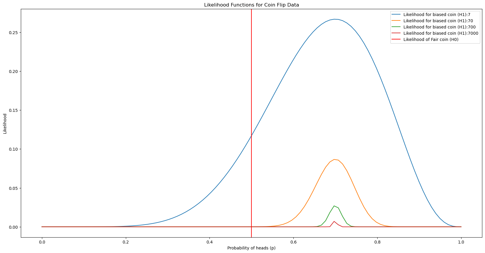
Note that, H0 is a vertical line whereas H1 is a continuous function (as alternate hypothesis considers all the probabilities of head between 0 and 1.

Let’s now look at how these behave as number of heads change from 1 to 9 out of total 10 tosses. We can clearly see how the distribution of alternate hypothesis gets skewed whereas it appears as a normal distribution when we get 5 out of 10 tosses at head.

Let’s now look at the posterior probabilities of null and alternate hypothesis in each of the above cases:

For our observation: we can clearly see that we do not have enough evidence to say that coin is biased as the P(H0) > P(H1).

Adding snippet for the above segment of code as well:

plt.figure(figsize=(20,10))
for observed_heads in range(1,total_flips): 
    plt.plot(p_values, [binom.pmf(observed_heads, total_flips, p) for p in p_values], 
             label='Likelihood for biased coin (H1):{}'.format(observed_heads))
    plt.xlabel('Probability of heads (p)')
    plt.ylabel('Likelihood')
    plt.title('Likelihood Functions for Coin Flip Data')
    
plt.axvline(0.5, color='r', linestyle='-', label='Likelihood of Fair coin (H0)')
plt.legend()
plt.show()


h0 = {}
h1 = {}

for observed_heads in range(1,total_flips): 
    total_flips = 10

    # Now lets compute the likelihood of null hypothesis conditional on 
    # this is where discussion related to binomial distribution mentioned above is
    # helpful
    likelihood_h0 = binom.pmf(observed_heads, total_flips, 0.5)

    # computing likelihood of alternate hypothesis is slightly tricky. 
    # here we assume that probaiblity of heads could be anything between 0 and 1.
    # but not .5 (why?)
    # we compute the mean likelihood given alternate hypothesis is true by 
    # computing the probability mass function value over the range p and taking
    # mean of that
    p_values = np.linspace(0, 1, 100)
    likelihood_h1 = np.mean([binom.pmf(observed_heads, total_flips, p) 
                            for p in p_values])

    # Let us now compute the marginal likelihood of observation which would be 
    # weighted sum of likelihoods where weights are probability of each 
    # hypothesis.
    marginal_likelihood = (likelihood_h0 * prior_h0) + (likelihood_h1 * prior_h1)

    # Now we can compute the posterior probabilities using definitons above.
    posterior_h0_explicit = (likelihood_h0 * prior_h0) / marginal_likelihood
    posterior_h1_explicit = (likelihood_h1 * prior_h1) / marginal_likelihood
    
    h0[observed_heads] = posterior_h0_explicit
    h1[observed_heads] = posterior_h1_explicit
    
import pandas as pd 
    
df_results = pd.DataFrame({'Posterior probability of H0 (fair coin)':h0,
              'Posterior probability of H1 (biased coin)':h1}).round(2)

df_results

What-If Analysis.

Now let’s take two interesting what if cases.

Case 1: What if we had 100 or 1000s of observations and has similar percentage of heads

In such a scenario probability of H1 would increase dramatically & let us prove that running simulations:

These results are so intuitive and tell us how the power of bayesian tests improve as number of observations improve. When number of samples re more, we need proportionately less number of observations to discard the null hypothesis.

Case 2: Lets us now consider if we had a prior information that there 80% chance that coin is biased instead of 50%.

In such a scenario, we need lesser number of samples as compared to the 50% case to reject the null hypothess. Let’s see this again with the help of a simulation:

In this table we can see that as the prior probability of alternate hypothesis increases, we need smaller number of of heads to prove that coin is biased. compare the cases of .5 vs .7 priors for h1 . in cases of .5, 7 heads give us posterior probability of coin being biased as .43 whereas in case of .7, posterior probability for same number of 7 heads increases to .64.

Future improvements

We could run more simulations and take rather complicated distributions to perform this test in future articles.

If you liked the explanation , follow me for more! Feel free to leave your comments if you have any queries or suggestions.

You can also check out other articles written around data science, computing on medium. If you like my work and want to contribute to my journey, you cal always buy me a coffee :)

buy me a coffee

Reference

[1] Github link to the code: https://github.com/girish9851/bayesian_hypothesis_testing/blob/main/bayesian_ht.ipynb

[2] https://en.wikipedia.org/wiki/Bayes%27_theorem

[3] https://www.probabilisticworld.com/calculating-coin-bias-bayes-theorem/