Deep Convolutional Generative Adversarial Networks

Deep Convolutional Generative Adversarial Networks — DCGAN is one of the first algorithms towards the Generative AI on Image data. In this article, we will break down the steps involved and provide a clear explanation of the algorithm.

Introduction

Imagine that you want to learn how to write letters used in a new language from scratch but there is no source to learn from. It’s definitely impossible to learn then, no?

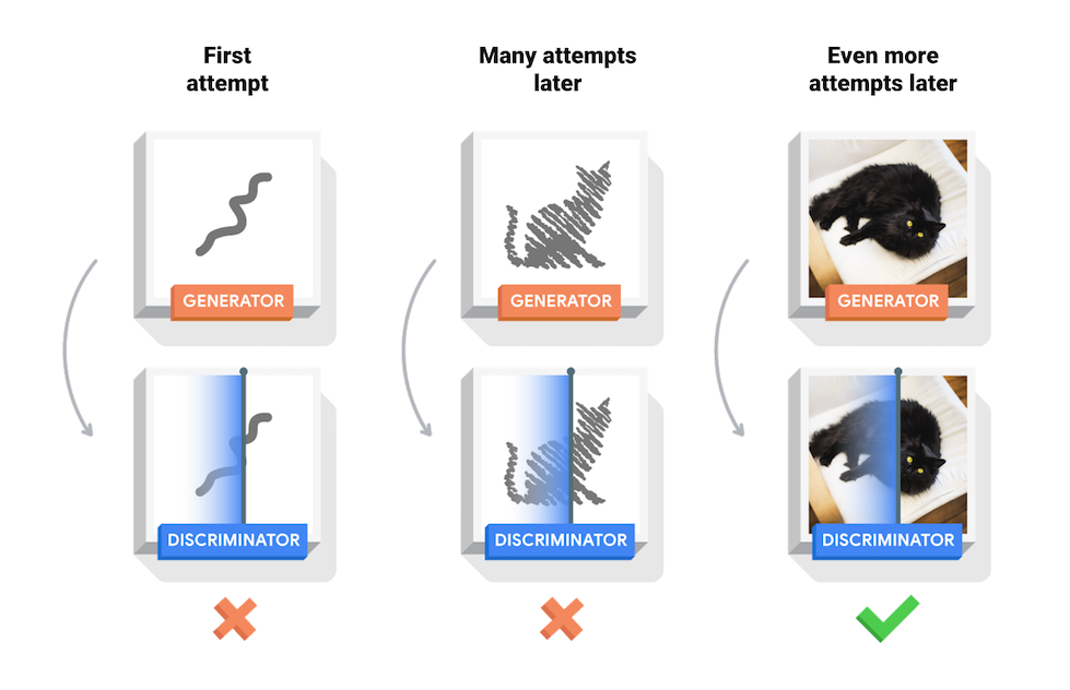
What if there is a teacher who provides you continuous feedback. You make some really random drawing and teacher provides you feedback depending on your drawing so that it gets you closer to the actual letter without exactly telling you what to draw. Then you draw letters again but this time utilizing the information provided to you by the teacher and using information in your initial drawing. You will surely improve albeit improvement pace will depend on various factors. This cycle goes on and eventually, you will get to a point where teacher would not have any feedback left because by then you would have learnt how to draw letters.

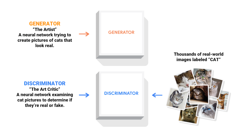
Generative Adversarial Networks work on a very similar principle where there is a generator which is generating images and a discriminator which is discriminating between the real and fake images. In example above, think of the fakes being generated by you while the actual letters are the real ones. If teacher is no more able to differentiate between the fake letters (drawn by you) and real letters (actual letters), then you have learnt how to draw letters.

Deep Convolutional Generative Adversarial Networks — a map showing the feedback loop of GAN; credit: https://towardsai.net/p/l/generative-ai-gans

Generator generates the images starting with random inputs and discriminator is trying to determine if the images are fake or real based on the real world training data of Cats. credit: https://www.tensorflow.org/tutorials/generative/dcgan

Using the continuous feedback from discriminator, generator improves gradually and results in almost a real picture of cat. credit: https://www.tensorflow.org/tutorials/generative/dcgan

Dataset

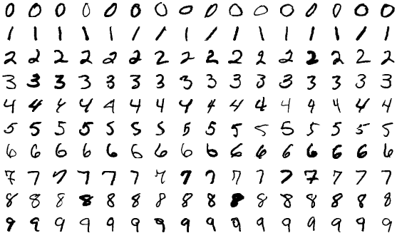
MNIST data is one of the go-to datasets for deep learning problems due to its simplicity and we will be utilizing it in this explanation.

Example of MNIST data, credit: https://en.wikipedia.org/wiki/MNIST_database

import tensorflow as tf

# To generate GIFs
!pip install imageio
# Install the 'imageio' library, used for generating GIFs.
!pip install git+https://github.com/tensorflow/docs
# Install the 'tensorflow/docs' library from its GitHub repository. 
# This library is used for documentation purposes.

import glob
import imageio
import matplotlib.pyplot as plt
import numpy as np
import os
import PIL
# Import various Python libraries and modules, 
# including glob (file manipulation), imageio (image processing),
# matplotlib.pyplot (plotting), numpy (numerical operations), 
# os (operating system interactions), and PIL (Python Imaging Library).

from tensorflow.keras import layers
# Import layers module from the TensorFlow.keras library, 
# which is used for creating neural network layers.
import time
# Import the time module for time-related operations.

from IPython import display
# Import the display module from IPython, 
# which is used for interactive display features in Jupyter Notebook.

(train_images, train_labels), (_, _) = tf.keras.datasets.mnist.load_data()
# Load the MNIST dataset using TensorFlow's built-in dataset loading function. 
# This dataset contains images of handwritten digits (0-9).

train_images = train_images.reshape(train_images.shape[0], \
                    28, 28, 1).astype('float32')
# Reshape the training images to have a shape of 
# (number of images, 28, 28, 1). 
# The 1 at the end indicates that the images are grayscale.

train_images = (train_images - 127.5) / 127.5
# Normalize the pixel values of the images to be in the range [-1, 1]. 
# This is a common practice in GANs (Generative Adversarial Networks).

BUFFER_SIZE = 60000
# Set the buffer size for shuffling the training data.
BATCH_SIZE = 256
# Define the batch size for training.

# Batch and shuffle the data
train_dataset = tf.data.Dataset.from_tensor_slices(train_images).\
                    shuffle(BUFFER_SIZE).batch(BATCH_SIZE)

# Create a TensorFlow dataset from the training images, 
# shuffle them with the specified buffer size, and 
# batch them with the defined batch size. 
# This dataset will be used for training our DCGAN model.

In above code snippet, we are doing the following:

Importing all the libraries
loading the MNIST data
rescaling the images, shuffling and creating batches for the training the DCGAN model.

Third step is very important to optimise our training.

Generator

def make_generator_model():
    # Create a function to build the generator model.

    model = tf.keras.Sequential()
    # Create a sequential model using TensorFlow's Keras API. 
    # This model will be used to generate synthetic images.

    model.add(layers.Dense(7*7*256, use_bias=False, input_shape=(100,)))
    # Add a fully connected layer (Dense) with 7*7*256 units, 
    # which takes a 100-dimensional random noise vector as input.
    # use_bias=False means no bias terms are used in this layer.

    model.add(layers.BatchNormalization())
    # Add a batch normalization layer to normalize the activations 
    # of the previous layer. Batch normalization helps stabilize training.

    model.add(layers.LeakyReLU())
    # Add a Leaky ReLU activation function to introduce non-linearity 
    # in the network.

    model.add(layers.Reshape((7, 7, 256)))
    # Reshape the output of the previous layers to have 
    # a shape of (7, 7, 256).
    # This is a common step in generator models.

    assert model.output_shape == (None, 7, 7, 256)
    # Check if the output shape matches the expected shape. 
    # 'None' represents the batch size, which can vary during training.

    model.add(layers.Conv2DTranspose(128, 
                (5, 5), strides=(1, 1), padding='same', use_bias=False))

    # Add a transposed convolutional layer (Conv2DTranspose) with 128 filters,
    # a kernel size of (5, 5), stride (1, 1), and 'same' padding.
    # use_bias=False means no bias terms are used in this layer.

    assert model.output_shape == (None, 7, 7, 128)
    # Check the output shape of this layer.

    model.add(layers.BatchNormalization())
    # Add another batch normalization layer for stabilization.

    model.add(layers.LeakyReLU())
    # Add Leaky ReLU activation.

    model.add(layers.Conv2DTranspose(64, (5, 5), strides=(2, 2), 
              padding='same', use_bias=False))
    # Add another transposed convolutional layer with 64 filters, 
    # larger stride (2, 2), and 'same' padding.

    assert model.output_shape == (None, 14, 14, 64)
    # Check the output shape of this layer.

    model.add(layers.BatchNormalization())
    # Add batch normalization.

    model.add(layers.LeakyReLU())
    # Add Leaky ReLU activation.

    model.add(layers.Conv2DTranspose(1, (5, 5), strides=(2, 2), 
              padding='same', use_bias=False, activation='tanh'))
    # Add a final transposed convolutional layer with 1 filter, 
    # larger stride (2, 2), and 'same' padding.
    # The activation function 'tanh' is used to ensure the output 
    # values are in the range [-1, 1], suitable for image data.

    assert model.output_shape == (None, 28, 28, 1)
    # Check the final output shape.

    return model
    # Return the complete generator model.

# Generate the generator model using above function
generator = make_generator_model()

# Create random noise by sampling from a 
# normal distribution with a shape of [1, 100].
noise = tf.random.normal([1, 100])

# Generate an image using the generator model by passing 
# the random noise as input.
# Set the training mode to False to ensure that the generator 
# doesn't update its parameters during this generation.
generated_image = generator(noise, training=False)

# Display the generated image using Matplotlib. 
# It's a grayscale image, so we specify the colormap as 'gray'.
plt.imshow(generated_image[0, :, :, 0], cmap='gray')

Generator model starts with a random input and it generates an image of 28x28 size. However, note that parameters need to be optimised to get a desired result. For example, the layers.Dense & layers.Conv2DTranspose steps define the tensors which contain the required parameters. Desired result from our generator model in this case would be MNIST quality integer images.

For this optimisation, we need to utilise the discriminator model. Discriminator takes an image of size 28x28 as an input and results in a probability of it being an integer. As you might have guessed, from getting to an image to probability of it being an integer, we again need parameters and optimisation of these parameters.

As we will see in next step both these trainings run in parallel for the epochs defined by us.

Discriminator

def make_discriminator_model():
    # Create a function to build the discriminator model.

    model = tf.keras.Sequential()
    # Create a sequential model using TensorFlow's Keras API. 
    # This model will be used to discriminate between real and fake images.

    model.add(layers.Conv2D(64, (5, 5), strides=(2, 2), padding='same', 
                    input_shape=[28, 28, 1]))
    # Add a convolutional layer with 64 filters, a kernel size of (5, 5), 
    # stride (2, 2), and 'same' padding.
    # input_shape specifies the input shape for the first layer, 
    # which is [28, 28, 1] for grayscale images.

    model.add(layers.LeakyReLU())
    # Add a Leaky ReLU activation function to introduce non-linearity 
    # in the network.

    model.add(layers.Dropout(0.3))
    # Add a dropout layer to help prevent overfitting by randomly setting 
    # a fraction of input units to 0 during training.

    model.add(layers.Conv2D(128, (5, 5), strides=(2, 2), padding='same'))
    # Add another convolutional layer with 128 filters and similar settings.

    model.add(layers.LeakyReLU())
    # Add Leaky ReLU activation.

    model.add(layers.Dropout(0.3))
    # Add another dropout layer.

    model.add(layers.Flatten())
    # Flatten the output of the convolutional layers into a 1D tensor.

    model.add(layers.Dense(1))
    # Add a dense layer with a single output unit. 
    # This layer will produce a scalar value 
    # representing the discriminator's decision.

    return model
    # Return the complete discriminator model.

# decision making step 
discriminator = make_discriminator_model()
decision = discriminator(generated_image)
print (decision)

Optimisers & Loss functions for Generator and Discriminator training

Before we proceed with training our generator and discriminator, we need to define loss functions which will determine how well our generator and discriminator is performing in their respective tasks. For the sake of clarity:

Discriminator’s loss function uses both MNIST images and images created by generator model in training data.
Generator’s loss function is purely based on the images created by it.

In both the cases, we are trying to solve a classification problem hence we are using cross entropy loss function. We utilise this loss function and gradient descent to update the parameters during the training process.

# Define a loss function for the discriminator using 
# binary cross-entropy loss.
# This loss function compares the discriminator's output 
# to ground truth labels.
cross_entropy = tf.keras.losses.BinaryCrossentropy(from_logits=True)

# Define the discriminator loss function, 
# which measures the error in classifying real and fake images.
def discriminator_loss(real_output, fake_output):
    # Compute the loss for real images by comparing them 
    # to a tensor of ones (real labels).
    real_loss = cross_entropy(tf.ones_like(real_output), 
                              real_output)
    # Compute the loss for fake images by comparing them to a 
    # tensor of zeros (fake labels).
    fake_loss = cross_entropy(tf.zeros_like(fake_output), 
                               fake_output)
    # Calculate the total discriminator loss by summing the real 
    # and fake losses.
    total_loss = real_loss + fake_loss
    return total_loss

# Define the generator loss function, 
# which measures the error in fooling the discriminator.
def generator_loss(fake_output):
    # Compute the loss by comparing the generator's output 
    # to a tensor of ones (indicating that the generator wants 
    # to fool the discriminator).
    return cross_entropy(tf.ones_like(fake_output), fake_output)

# Create optimizers for the generator and discriminator.
# These optimizers are used to update the neural network weights 
# during training.
generator_optimizer = tf.keras.optimizers.Adam(1e-4)
discriminator_optimizer = tf.keras.optimizers.Adam(1e-4)

# Define checkpointing for saving and restoring model weights during training.
# This allows you to resume training from a saved state.
checkpoint_dir = './training_checkpoints'
checkpoint_prefix = os.path.join(checkpoint_dir, "ckpt")
checkpoint = tf.train.Checkpoint(generator_optimizer=generator_optimizer,
                          discriminator_optimizer=discriminator_optimizer,
                                 generator=generator,
                                 discriminator=discriminator)

Training

In each training step:

We first calculate the loss function for the images.
This is followed by calculating the gradient of the loss function with respect to parameters in the model.
Next step is to use the optimiser to update parameters using the gradient information calculated in previous step.
We perform training for each of the defined batches and for the number of epochs defined so total no of times training step will run = epochs * number of batches in dataset.
For the illustration purposes, we also save the images in the intermediate steps which shows how our generator is getting better.

EPOCHS = 75
noise_dim = 100
num_examples_to_generate = 16

# Generate a fixed random seed for producing consistent images during training.
seed = tf.random.normal([num_examples_to_generate, noise_dim])

# Annotate the following function with `tf.function` to enable 
# TensorFlow's autograph feature, which compiles the function 
# for better performance.
@tf.function
def train_step(images):
    # Generate random noise for the batch of images.
    noise = tf.random.normal([BATCH_SIZE, noise_dim])

    # Use gradient tapes to record operations for gradient calculation.
    with tf.GradientTape() as gen_tape, tf.GradientTape() as disc_tape:
        # Generate fake images using the generator model.
        generated_images = generator(noise, training=True)

        # Calculate the discriminator's outputs for both real and fake images.
        real_output = discriminator(images, training=True)
        fake_output = discriminator(generated_images, training=True)

        # Compute generator and discriminator losses.
        gen_loss = generator_loss(fake_output)
        disc_loss = discriminator_loss(real_output, fake_output)

    # Calculate gradients of the losses with respect 
    # to the trainable variables of the generator and discriminator.
    gradients_of_generator = gen_tape.gradient(gen_loss, 
                                               generator.trainable_variables)
    gradients_of_discriminator = disc_tape.gradient(disc_loss, 
                                               discriminator.trainable_variables)

    # Apply gradients to update the generator and 
    # discriminator using their respective optimizers.
    generator_optimizer.apply_gradients(zip(gradients_of_generator, 
                                        generator.trainable_variables))
    discriminator_optimizer.apply_gradients(zip(gradients_of_discriminator, 
                                        discriminator.trainable_variables)

# Define a training loop for the GAN model.
def train(dataset, epochs):
    for epoch in range(epochs):
        start = time.time()

        # Iterate over the dataset and perform training steps.
        for image_batch in dataset:
            train_step(image_batch)

        # Produce images for monitoring the training progress.
        display.clear_output(wait=True)
        generate_and_save_images(generator, epoch + 1, seed)

        # Save the model's checkpoint every 15 epochs.
        if (epoch + 1) % 15 == 0:
            checkpoint.save(file_prefix = checkpoint_prefix)

        print ('Time for epoch {} is {} sec'.format(epoch + 1, 
                    time.time()-start))

    # Generate and display images after the final epoch.
    display.clear_output(wait=True)
    generate_and_save_images(generator, epochs, seed)

# Generate and save images using the generator model for visualization.
def generate_and_save_images(model, epoch, test_input):
    # Set the `training` flag to False to run the model in 
    # inference mode (batch normalization behaves differently).
    predictions = model(test_input, training=False)

    # Create a 4x4 grid to display generated images.
    fig = plt.figure(figsize=(4, 4))

    for i in range(predictions.shape[0]):
        plt.subplot(4, 4, i+1)
        plt.imshow(predictions[i, :, :, 0] * 127.5 + 127.5, cmap='gray')
        plt.axis('off')

    # Save the figure with generated images for this epoch.
    plt.savefig('image_at_epoch_{:04d}.png'.format(epoch))
    plt.show()

We execute the training and save the gif of images created in each step for illustrating the progress.

# Train the GAN using the specified training dataset and number of epochs.
train(train_dataset, EPOCHS)

# Restore the latest checkpoint to resume training or generate images.
checkpoint.restore(tf.train.latest_checkpoint(checkpoint_dir))

# Define a function to display a single image based on the epoch number.
def display_image(epoch_no):
    return PIL.Image.open('image_at_epoch_{:04d}.png'.format(epoch_no))

# Define the name of the animated GIF file to be generated.
anim_file = 'dcgan.gif'

# Create an imageio writer to generate the animated GIF.
with imageio.get_writer(anim_file, mode='I') as writer:
    # Get a list of image filenames that match the naming pattern.
    filenames = glob.glob('image*.png')
    # Sort the filenames to ensure the images are in the correct order.
    filenames = sorted(filenames)
    # Iterate through the sorted filenames and append each image to the GIF.
    for filename in filenames:
        image = imageio.imread(filename)
        writer.append_data(image)
    # Append the last image one more time to create a smooth 
    # loop in the animation.
    image = imageio.imread(filename)
    writer.append_data(image)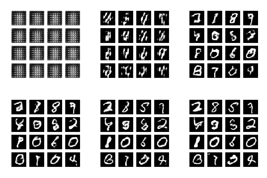

Gif showing how our generator got better with each epoch

Conclusion

In the article above, we went through a simple tutorial implementing deep convolutional generative adversarial networks which uses generator and discriminator models to provide continuous feedback and improvments in generator. This algorithm is one of the first among the GAN models and provide a good insight into how generative AI on image data works.

References

If you found the explanation helpful, follow me for more content! Feel free to leave comments with any questions or suggestions you might have.

You can also check out other articles written around data science, computing on medium. If you like my work and want to contribute to my journey, you cal always buy me a coffee :)

Artificial Intelligence

Search This Blog

Indie Quant