Text Classification Using Recurrent Neural Networks

Supervised learning problems are one of the core areas of interest in machine learning space. There are a range of approaches available to solve such a problem. In this article, we will delve into the details of a text classification problem and explore how text classification using Recurrent Neural Networks can be used to address it.

Introduction

Text classification is one of the most popular problems in natural language processing (NLP) and machine learning. In this problem, we are provided with text data and our goal is to find out the class of the text from predefined categories or labels. This has myriad of utilities such as organizing documents/texts, analyzing and being able to comment on a data without going through the whole text. It can also help us in making business decisions such as directing a customer query or issue to correct department. This problem statement finds applications in areas such as spam detection, and topic categorization etc. as well.

Text classification finds its most common use in automatically identifying phishing/spam mails

On a high level, all such categorizations have these three steps:

• Text Data (Input) : Raw text data such as movie reviews or emails.
• Model (Machine Learning/Deep Learning): The model learns patterns from the text data.
• Output (Model assigned categories): Categorized text such as positive or negative sentiment or spam or non- spam data.

IMBD Dataset

The IMDB reviews dataset is a popular resource used for text classificationtasks. This dataset includes reviews from IMDB and each review is labeled as either “positive” or “negative.” We will be using this dataset in this article to design and evaluate our text classification model.

Example:

Review 

This was an absolutely terrible movie.
Don't be lured in by Christopher Walken or Michael Ironside.
Both are great actors, but this must simply be their worst role in history.
Even their great acting could not redeem this movie's ridiculous storyline.
This movie is an early nineties US propaganda piece.
The most pathetic scenes were those when the Columbian
rebels were making their cases for revolutions.
Maria Conchita Alonso appeared phony,
and her pseudo-love affair with Walken
was nothing but a pathetic emotional plug in a
movie that was devoid of any real meaning.
I am disappointed that there are movies like this,
ruining actor's like Christopher Walken's good name.
I could barely sit through it.

Class 

Negative

Data Processing

High level steps required in processing data

Loading data: To begin with, we need to load the IMDb reviews dataset using TensorFlow Datasets (TFDS). This dataset provides a collection of movie reviews along with sentiment labels (positive or negative).

After loading the dataset, it is divided into training and testing sets:

• Training and Testing Sets: The dataset is split into train_dataset for training the model and test_dataset for evaluating the model’s performance.

Processing & associated optimization: to ensure efficient and effective training we define buffer size & batch size:

• Buffer Size: Set using BUFFER_SIZE = 10000. Buffer size defines the size of the buffer used for shuffling the dataset. Higher buffer size improves the randomness of shuffling but requires more memory.
• Batch Size: BATCH_SIZE = 64. Batch size determines how many examples are processed together in one batch during training.

Training dataset prep: training data is prepared by using following steps

• Shuffle — data set is shuffled to randomize the order of examples.
• Batch — It is then divided into batches of specified sizes.
• Prefetch — To improve performance, we load the next batch while current batch is in process.

Test dataset prep: test dataset prep follows the same steps except shuffling the data (this is not required; why?)

• Batch: The test dataset is batched into chunks of the specified size.
• Prefetch: Prefetching is also applied to enhance performance.

Text Vectorization and Encoding

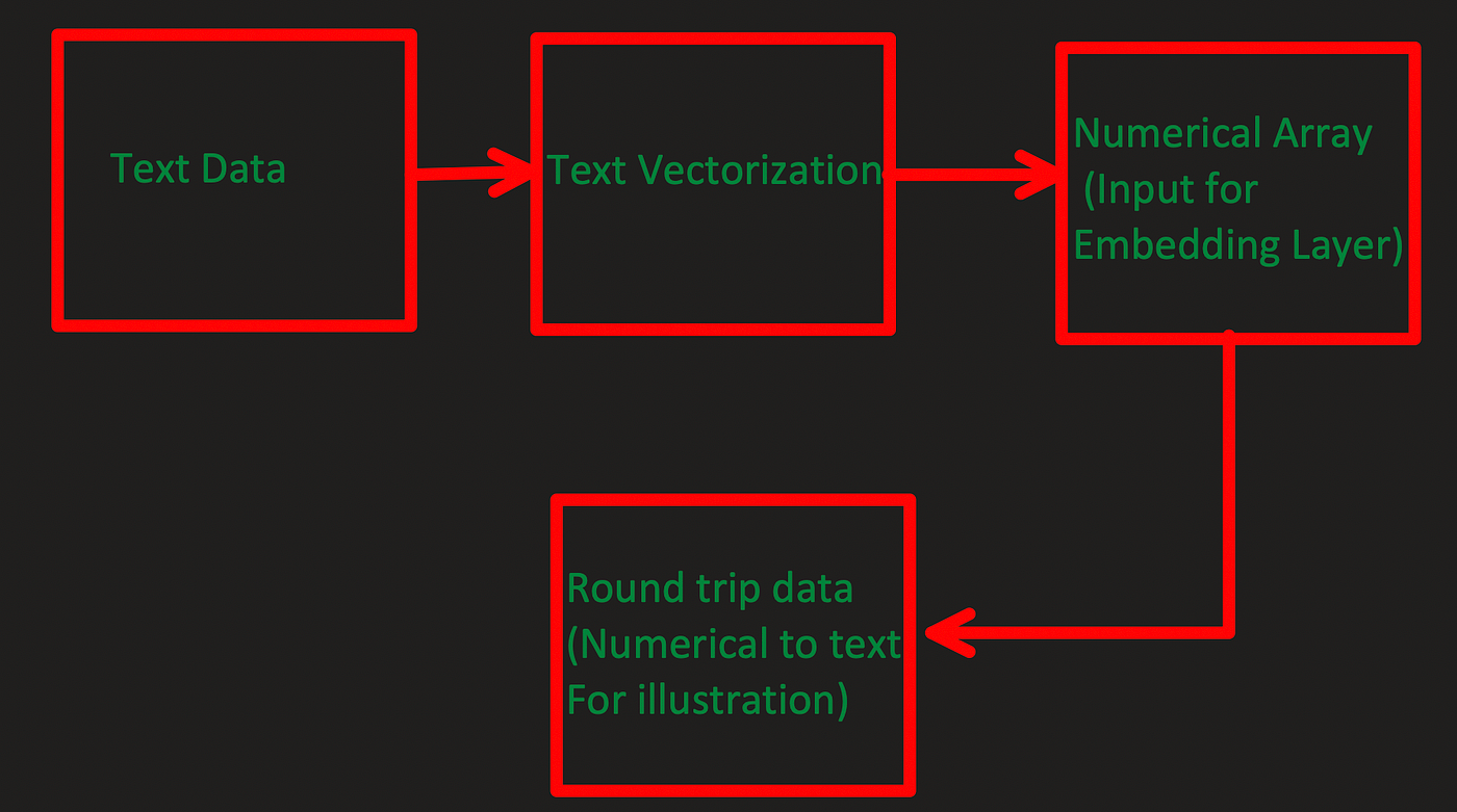
We need to convert text data to numerical data so that it can be fed to the model. We start by defining the unique tokens (words) allowed in the text vectorization process. We then pass the text data through this text vectorizer to convert text data to array of integers.

Steps

Example

Below example shows the input and after round trip text. Round trip refers to passing input through text vectorizer and converting it back to text data.

Original:  b"I just saw this film in Santa Barbara. 
My friend knew someone who worked on it, so i thought i'd check it out. 
i thought it was a really beautiful film and cant wait to go look at it again. 
the actors were really good and i loved all the music! 
there was not a lot of talking in the film, 
which at first felt a little strange- but once i got into it, 
i thought that the story and the acting was really emotional and meaningful 
and thought that it left a lot to the imagination. 
i want to see the movie again because there was so much going on in it that 
i forgot a lot of small things, but know that i left the theater 
thinking about the film. it was shot beautifully and the whole thing was 
really unique."


Round-trip:  i just saw this film in [UNK] [UNK] my friend knew someone who 
worked on it so i thought id check it out i thought it was a really beautiful
 film and cant wait to go look at it again the actors were really good and 
i loved all the music there was not a lot of talking in the film which at 
first felt a little strange but once i got into it i thought that the story
 and the acting was really emotional and [UNK] and thought that it left a 
lot to the [UNK] i want to see the movie again because there was so much 
going on in it that i [UNK] a lot of small things but know that i left the 
theater thinking about the film it was shot [UNK] and the whole thing was 
really unique

BiLSTM with Attention Model to Predict Missing Characters in a Word

In this article, we will go through one of the approaches to predict missing characters in a word. This approach is…

medium.com

Code

# Importing the NumPy library for numerical operations
import numpy as np
# Importing TensorFlow Datasets (tfds) for easy access to standard datasets
import tensorflow_datasets as tfds
# Importing TensorFlow for building and training machine learning models
import tensorflow as tf
# Disabling the progress bar that is displayed during TensorFlow Datasets operations
tfds.disable_progress_bar()
# Importing the pyplot module from matplotlib for creating visualizations
import matplotlib.pyplot as plt
# Define a function to plot the training and validation metrics


def plot_graphs(history, metric):
    # Plot the training metric values from the history object
    plt.plot(history.history[metric])
    # Plot the validation metric values from the history object
    plt.plot(history.history['val_'+metric], '')
    # Label the x-axis as "Epochs"
    plt.xlabel("Epochs")
    # Label the y-axis with the name of the metric
    plt.ylabel(metric)
    # Add a legend to differentiate between the training and validation metrics
    plt.legend([metric, 'val_'+metric])


# Load the IMDb reviews dataset from TensorFlow Datasets
# - `with_info=True` includes dataset metadata
# - `as_supervised=True` returns the dataset i/n a (input, label) tuple format
dataset, info = tfds.load('imdb_reviews', with_info=True, as_supervised=True)
# Split the dataset into training and testing sets
train_dataset, test_dataset = dataset['train'], dataset['test']
# Display the structure of the elements in the training dataset
# This shows the data type and shape of the input and label tensors
display(train_dataset.element_spec)


for example, label in train_dataset.take(1):
    print('text: ', example.numpy())
    print('label: ', label.numpy())

# Set the buffer size for shuffling the dataset
# Larger buffer size results in better shuffling but requires more memory
BUFFER_SIZE = 10000
# Set the batch size for processing the data
# Each batch will contain this number of examples
BATCH_SIZE = 64
# Prepare the training dataset:
# - Shuffle the dataset with the specified buffer size to randomize the order of examples
# - Batch the dataset into chunks of the specified batch size
# - Prefetch data to improve performance by loading the next batch while the current batch is being processed
train_dataset = train_dataset.shuffle(BUFFER_SIZE).batch(BATCH_SIZE).prefetch(tf.data.AUTOTUNE)
# Prepare the test dataset:
# - Batch the dataset into chunks of the specified batch size
# - Prefetch data to improve performance by loading the next batch while the current batch is being processed
test_dataset = test_dataset.batch(BATCH_SIZE).prefetch(tf.data.AUTOTUNE)
# Iterate through the training dataset and take the first batch for inspection
# - `example` contains the input text data
# - `label` contains the corresponding labels
for example, label in train_dataset.take(1):
    # Print the first three examples from the batch
    # Convert tensors to numpy arrays for easier inspection
    print('texts: ', example.numpy()[:3])
    # Print an empty line for separation
    print()
    # Print the first three labels from the batch
    # Convert tensors to numpy arrays for easier inspection
    print('labels: ', label.numpy()[:3])
    # Define the maximum vocabulary size for the TextVectorization layer
    # This determines the number of unique tokens the encoder will consider

VOCAB_SIZE = 1000
# Initialize a TextVectorization layer with a maximum of VOCAB_SIZE unique tokens
# This layer will convert text data into integer sequences based on the vocabulary
encoder = tf.keras.layers.TextVectorization(
max_tokens=VOCAB_SIZE)
# Fit the TextVectorization layer to the training dataset
# This process builds the vocabulary from the text data in the training set
# The lambda function extracts only the text part from the (text, label) tuple
# The `.adapt` method creates the vocabulary for the layer. Here are the first 20 tokens in the vocabulary.
# After accounting for padding and unknown tokens, these tokens are listed in order of how frequently they appear.
encoder.adapt(train_dataset.map(lambda text, label: text))
# Retrieve the vocabulary as a NumPy array
# This contains the words (tokens) corresponding to the integer indices
vocab = np.array(encoder.get_vocabulary())
# Display the first 20 words in the vocabulary
# These are the most frequent tokens found in the training data
display('First 20 words in the vocabulary: ', vocab[:20])
# Encode the first 3 examples from the batch using the TextVectorization layer
# This converts the text data into sequences of integer indices based on the vocabulary
encoded_example = encoder(example)[:3].numpy()
# Display the encoded integer sequences for the first 3 examples
display(encoded_example)
# Print the original text and its round-trip encoding for the first 3 examples

for n in range(3):
    # Print the original text example
    print("Original: ", example[n].numpy())
    # Convert the encoded integer sequence back to text using the vocabulary
    # The vocabulary array maps integer indices back to words
    print("Round-trip: ", " ".join(vocab[encoded_example[n]]))
    # Print an empty line for separation
    print()

Sentiment Analysis using Deep Learning (BERT)

Sentiment analysis is one of the classic machine learning problems which finds use cases across industries. For…

medium.com

Model

As the article subject states, we are going to use recurrent neural network to perform text classification. Let’s try to understand what is RNN:

Recurrent neural networks (RNNs) are the kind of neural networks which are specifically designed to handle sequential information. Unlike traditional feedforward networks, RNNs have backward connections. This allows RNNs to retain the memory of previously seen inputs. This feature makes RNNs particularly effective for sequential problems such as speech modeling, time series prediction, and speech recognition.

However, RNNs do struggle because of issues such as vanishing and exploding gradients as well as difficulty in retaining long term dependencies. Advanced techniques, such as long-term and short-term memory networks (LSTM) and gated repeating units (GRUs), have been developed to overcome these challenges and increase performance.

In our modeling, we will be using Bidirectional LSTM which is a variant of RNN which particularly handles long term dependencies problem as it tries to retain context generated due to reading inputs forward and backward way.

We use below model architecture as our first model. As we can see, we are passing the text data through vectorizer which then is fed into embedding layer. Embedding layer is helpful in generating semantic representations, speeding up training and helps in generalization. This is followed by a layer of BiLSTM with 128 units which is then followed by a dense layer.

In the code, we also see how we are using padding and masking at the same time to handle different sizes of reviews.

Model Architecture

# Build a Sequential model using TensorFlow Keras
model = tf.keras.Sequential([
    # Encoder layer to convert text to token indices
    encoder,
    
    # Embedding layer to convert token indices to dense vectors
    # - input_dim: Size of the vocabulary (number of unique tokens)
    # - output_dim: Dimension of the dense embedding vectors
    # - mask_zero: Allows the layer to handle variable-length sequences by masking zeros
    tf.keras.layers.Embedding(
        input_dim=len(encoder.get_vocabulary()),  # Size of the vocabulary
        output_dim=64,  # Dimension of the embedding vectors
        mask_zero=True  # Enable masking for variable-length sequences
    ),
    
    # Bidirectional LSTM layer processes sequences in both forward and backward directions
    # - LSTM units: 64
    tf.keras.layers.Bidirectional(tf.keras.layers.LSTM(64)),
    
    # Dense layer with ReLU activation for additional processing
    # - Units: 64
    tf.keras.layers.Dense(64, activation='relu'),
    
    # Final Dense layer for producing the output
    # - Units: 1 (e.g., for binary classification or regression)
    tf.keras.layers.Dense(1)
])


##### Padding standardizes sequence lengths by adding extra values.
##### Masking allows the model to ignore these padding values during processing.

# Check which layers in the model support masking
# This helps determine if the model can properly handle padded sequences
print([layer.supports_masking for layer in model.layers])

# Predict on a sample text without padding
# Sample text is a straightforward example for model prediction
sample_text = ('The movie was cool. The animation and the graphics '
               'were out of this world. I would recommend this movie.')
# Convert the sample text into a NumPy array and ensure the type is 'object'
# `astype(object)` is used to handle the text data correctly
predictions = model.predict(np.array([sample_text]).astype(object))
# Print the prediction for the sample text
print(predictions[0])

# Predict on a sample text with padding
# Create a long padding string to simulate a sequence with extra length
padding = "the " * 2000
# Predict on both the sample text and the padded text
# Convert both texts into a NumPy array and ensure the type is 'object'
predictions = model.predict(np.array([sample_text, padding]).astype(object))
# Print the prediction for the sample text (only the first prediction)
print(predictions[0])

#### compiling the model 

model.compile(loss=tf.keras.losses.BinaryCrossentropy(from_logits=True),
              optimizer=tf.keras.optimizers.Adam(1e-4),
              metrics=['accuracy'])


# Train the model using the training dataset and validate with the test dataset
# - `train_dataset`: The dataset used for training the model
# - `epochs=10`: The number of epochs to train the model
# - `validation_data=test_dataset`: The dataset used for validating the model during training
# - `validation_steps=30`: The number of steps (batches) to draw from the validation dataset for evaluation

history = model.fit(train_dataset, epochs=10,
                    validation_data=test_dataset,
                    validation_steps=30)


# Evaluate the model on the test dataset
# - `test_dataset`: The dataset used for testing the model's performance
# The method returns the loss value and metrics specified during model compilation (e.g., accuracy)
test_loss, test_acc = model.evaluate(test_dataset)

# Print the loss value obtained on the test dataset
# This represents how well the model performed on the test data, with lower values indicating better performance
print('Test Loss:', test_loss)

# Print the accuracy value obtained on the test dataset
# This represents the proportion of correct predictions made by the model on the test data
print('Test Accuracy:', test_acc)

# Import the `plot_model` function from TensorFlow Keras utilities
from tensorflow.keras.utils import plot_model

# Generate and save a visual representation of the model architecture
plot_model(model,
            # Show the shapes of the layers' outputs in the diagram
            show_shapes=True,
            # Display the data types of the layers in the diagram
            show_dtype=True,
            # Show the names of the layers in the diagram
            show_layer_names=True,
            # Set the direction of the plot: 'TB' means top-to-bottom
            rankdir='TB',
            # Expand nested models (models within models) in the diagram
            expand_nested=True,
            # Set the resolution of the image
            dpi=50,
            # Display the activation functions used in the layers
            show_layer_activations=True,
            # Indicate which layers are trainable in the diagram
            show_trainable=True)

Training & Results

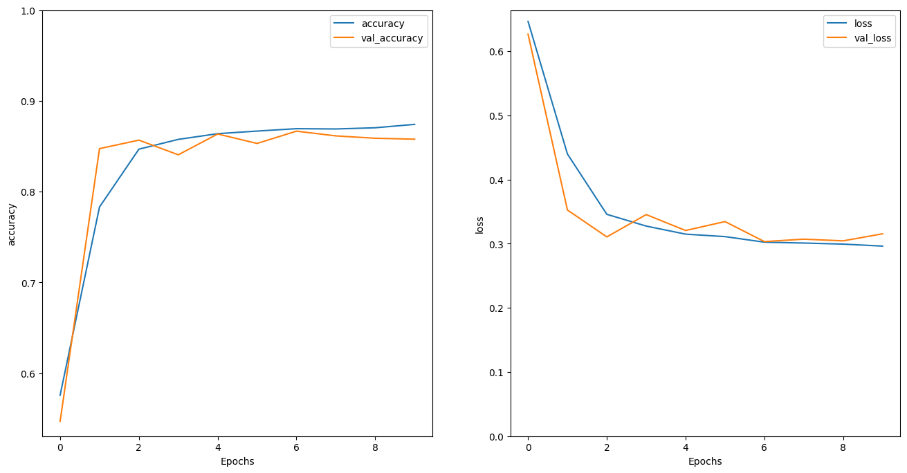
As shown in above code snippet, we train the model with Adam optimizer & BinaryCrossentropy loss function. Since, it’s a classification problem, we are going with “accuracy” as metric.

We can see that we achieve 88% validation accuracy after 10 epochs. This performance is really good given we have very long reviews and language could be confounding for some. This high accuracy is primarily due to the BiLSTM layer which is able to learn much more context than traditional RNN.

An Intuitive Approach to Time-Series Clustering

We will use silhouette score and few distance metrics to perform experiments on time-series clustering while leveraging…

medium.com

Model with two BiLSTM layers

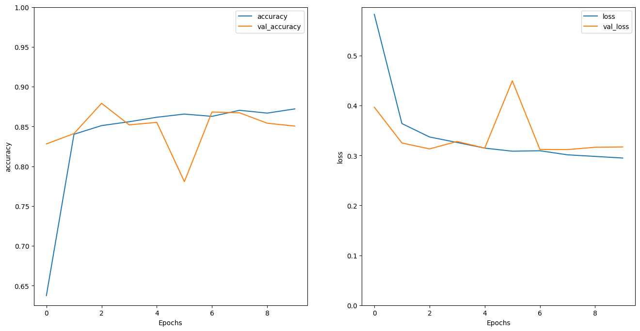
Let us explore if we could perform better by adding one more layer of BiLSTM. The updated architecture is shown below. Notice the second bidirectional layer, with this additional layer we have two BiLSTM layers with 128 units each.

Model 2 Architecture

Below result show that model performance has not improved by adding another 128 units BiLSTM. Validation accuracy hovers around 85 % which is lower than our initial model.

Introduction to BIRCH Clustering & Python Implementation

Introduction to Clustering & need for BIRCH

python.plainenglish.io

Future Work & Conclusion

In this article, we went through text classification problem and how we can model it with the help of RNNs using tensorflow. We observed that BiLSTM is indeed good at learning context which results in a high validation accuracy for the single layered model.

We do feel that model can be further improved with more involved text processing ( for example: more VOCAB size) & hyper-parameter tuning of the model (such as no of units in BiLSTM layer, no of layers, addition of drop out layer etc.). You can read more about how to perform these parameter tunings from my other article which is around predicting missing characters in a word using BiLSTM (Link).

If you liked the explanation , follow me for more! Feel free to leave your comments if you have any queries or suggestions.

You can also check out other articles written around data science, computing on medium. If you like my work and want to contribute to my journey, you cal always buy me a coffee :)

buy me a coffee

References

1. [Datasets and TensorFlow APIs ] https://www.tensorflow.org/resources/models-datasets
2. [BiLSTM] : https://www.youtube.com/watch?v=_bt9OaavkT4
3. [BiLSTM vs LSTM] : https://medium.com/@souro400.nath/why-is-bilstm-better-than-lstm-a7eb0090c1e4
4. [Text Classification using BERT] https://medium.com/@girish9851/sentiment-analysis-using-deep-learning-bert-adf975232da2
5. [Github Link to Notebook] https://github.com/girish9851/Text-Classification-Using-RNN/blob/main/text-classification-using-rnn-2.ipynb