Handling Overfitting in Machine Learning
Handling Overfitting in Machine Learning
Overfitting is one of the key challenges in Machine Learning. This occurs when model performance on training data is significantly better than unseen data which implies that instead of learning general patterns about the data, model learnt about the noise or anomalies specific to training data. In this article, we will learn about the ways to detect & prevent overfitting.
What is overfitting?

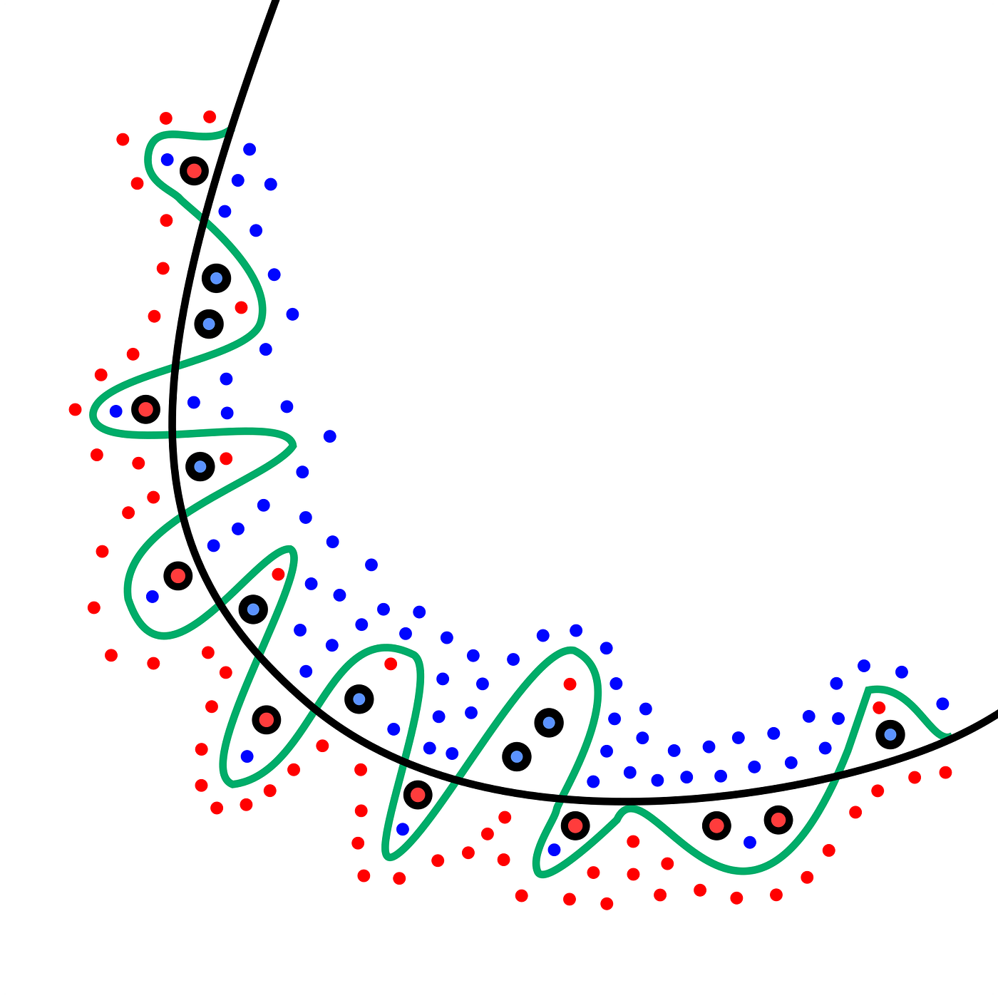
As shown in the graph above, if a model learns about the patterns specific to training data — such as wavy green line in this case — there is a good possibility that it will not perform as good on test data since pattern is not general enough. Now take the example of black line — chances of black line being a general trend is very high. We can also say that even though variance of error in green line would be low — it will have a significant bias.
How to Identify Overfitting?
1. Performance on training set & validation/test set
We can track the model performance on training and testing data. If model performs well on training data but have a poor performance on test data. This indicates that model is overfitting because it has memorized the training data instead of learning a general pattern which would have resulted in similar performance in both training and testing data.
How to prevent overfitting?
1. K-Fold cross validation

Before training the model and using it on test data, we can perform an optimization. For this optimization, we use k-fold cross-validation wherein training data is divided into k subsets. The model is trained on k-1 subsets and validated on the remaining subset. This process is repeated k times. We then observe the average score across the k folds.
Instead of using the complete training data in first go if we use k fold cross validation — we can build an understanding on how a certain model might perform on test data since since during the k fold cross validation we are alway training on k-1 folds and we are computing score on left out subset.
from sklearn.model_selection import KFold, cross_val_score
from sklearn.ensemble import RandomForestClassifier

# Example data
X, y = load_data() # Load your dataset
kf = KFold(n_splits=5)

model = RandomForestClassifier()
scores = cross_val_score(model, X, y, cv=kf)
print("Cross-Validation Scores:", scores)
Pros:
• Provides a better estimate of model performance.
• Helps in utilizing the dataset efficiently.
Cons:
• Since we are building model & computing score k times — it’s computationally expensive, especially with large datasets.
• Might still overfit if not combined with other techniques.
2. Regularization

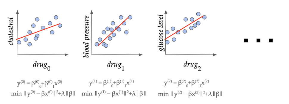
Using regularization, we put constraints on model parameters which prevents them to becoming too large or very complex. Few examples are Lasso & Ridge regression.
In Lasso (L1)regression, we add penatlies equal to the absolute value of coefficients which might result in some coefficients becoming exactly zero. Whereas in Ridge (L2) regression, square of coefficients are added as penalties. Ridge regression lowers the coefficient value as a result of the penalty for less important variables. However, one limitation is a hypter parameter called alpha which represents the strength of regularization needs to be tuned.
Example — Using Lasso and Ridge regularization in linear regression:
from sklearn.linear_model import Lasso, Ridge

# Lasso regression
lasso = Lasso(alpha=0.1) # Adjust alpha for regularization strength
lasso.fit(X_train, y_train)

# Ridge regression
ridge = Ridge(alpha=0.1)
ridge.fit(X_train, y_train)
Pros:
• Helps in reducing model complexity by penalizing large coefficients.
• Effective in feature selection (especially L1).
Cons:
• Requires tuning of the regularization parameter.
• Might under fit if regularization is too strong.
3. Pruning (for Decision Trees)

If we let a decision tree grow to full depth for each instance— its likely that decision tree will overfit. This is because tree will have a lot of branches. Large number of branches indicate that instead of learning general patterns in the data — we are also learning minor fluctuations in the training data. Additionally, large number of branches might also increase the model complexity without improving generalization.
Pruning can also be thought as a form of regularization which penalizes the complexity of the tree and hence avoids the excessive tree growth.
Example — Post-pruning a decision tree by removing nodes that provide little power in predicting the target variable:
from sklearn.tree import DecisionTreeClassifier

# Create and fit the model
dtree = DecisionTreeClassifier(max_depth=5) # Limit depth to prevent overfitting
dtree.fit(X_train, y_train)
Pros:
• Reduces the complexity of the model.
• Helps improve model interpretability.
Cons:
• May lose important information if not done correctly.
• Can require experimentation to find the optimal depth.
4. Dropout (for Neural Networks)

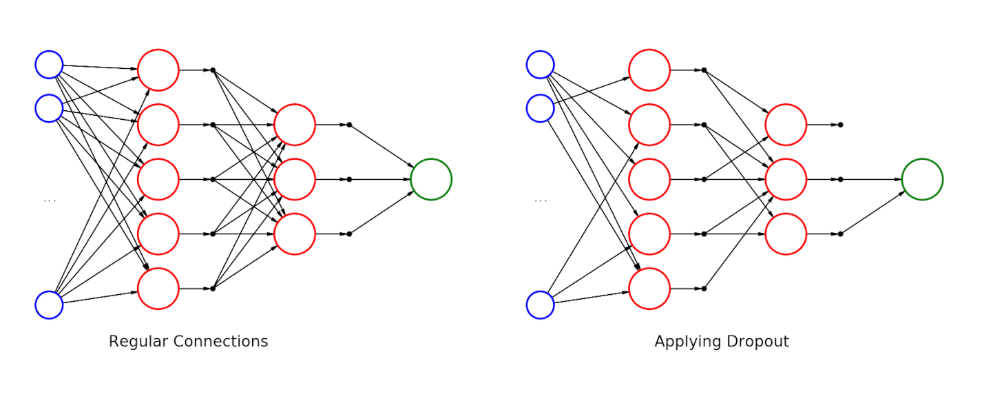
Dropout is a regularization method which applies specifically to neural networks & prevents overfitting. In dropout method, a proportion of neurons (units)is “dropped out” (i.e., setting to zero) during each training step. This prevents the network from becoming dependent on specific neurons and forces it to learn more robust and generalized patterns. By doing so, dropout layers in a neural network reduces overfitting & allows the model to generalize better to new, unseen data.
Example — Applying dropout during training to randomly set a fraction of input units to zero:
from tensorflow.keras.models import Sequential
from tensorflow.keras.layers import Dense, Dropout

model = Sequential()
model.add(Dense(64, activation='relu', input_shape=(input_dim,)))
model.add(Dropout(0.2)) # 50% dropout
model.add(Dense(1, activation='sigmoid'))

model.compile(loss='binary_crossentropy', optimizer='adam', metrics=['accuracy'])
model.fit(X_train, y_train, epochs=10)
Pros:
• Reduces overfitting in neural networks effectively.
• Can improve generalization by forcing the model to learn redundant representations.
Cons:
• May require additional tuning for dropout rates.
• Slower training due to the random dropping of neurons.
Future Work & Conclusion
This article is just some of the overfitting prevention methods. While many more exist — it would also be worthwhile to look into nuances of each technique in while implementing in real life problems. We will look delve deeper into each topic in upcoming artciles. Please comment on which one I should start with.
If you liked the explanation , follow me for more! Feel free to leave your comments if you have any queries or suggestions.
You can also check out other articles written around data science, computing on medium. If you like my work and want to contribute to my journey, you cal always buy me a coffee :)

References
[1] https://en.wikipedia.org/wiki/Dilution_%28neural_networks%29
[2] https://en.wikipedia.org/wiki/Decision_tree_pruning
[3] https://blog.ml.cmu.edu/2024/04/12/how-to-regularize-your-regression/
[4] https://www.geeksforgeeks.org/cross-validation-machine-learning/


Comments
Post a Comment