Introduction to BIRCH Clustering & Python Implementation

Clustering is one of the most used unsupervised machine learning techniques for finding patterns in data. Most popular algorithms used for this purpose are K-Means/Hierarchical Clustering. These algorithms do not adequately address problems of processing large datasets with limited amount of resources (i.e. memory and cpu). This is where BIRCH comes in picture and improves performance vis-a-vis aforementioned algorithms.

Source: sklearn

Balanced Iterative Reducing and Clustering using Hierarchies aka BIRCH deals with the large dataset problem described above by first creating a summary of data while retaining much of the distribution related information and then clustering the summary. Second step of BIRCH can use any of the clustering methods.

Flowchart of steps followed in algorithm

Source: research paper[1]

Following is a high level description of the algorithm:

For more details on the detailed algorithm nuances, you can refer to the associated research paper.

Implementation

Let’s now try to implement BIRCH on a dummy dataset and examine its performance vis-a-vis K-Means.

Dataset

We will be using dummy data created using sklearn library. Note that we are taking a simple case to illustrate implementation and comparison with K-Means. As the code snippet suggests, we are generating data with 10000 samples, 3 features and 6 Clusters with 1.5 cluster standard deviation. Let’s observe data characteristics visually in next section.

################### Common Libraries #################
import pandas as pd
import numpy as np
from time import time######## Data & Visualization Libraries ##############
from matplotlib import pyplot as plt
import seaborn as sns
sns.set()
from mpl_toolkits.mplot3d import Axes3D
from sklearn import datasets########## ML & datasets Libraries ###################
from sklearn.datasets import make_blobs
from sklearn.cluster import Birch
from sklearn.cluster import KMeans
from sklearn import metrics##################### Dataset ########################X, clusters = make_blobs(n_samples=10000,
                         n_features=3, 
                         centers=6, 
                         cluster_std=1.5, 
                         random_state=0)

Data Exploration

The scatter plot below shows relationship among variables. Clearly, there are 6 clusters with most of them separated out quite well.

########################## 3D scatter plot ###############
fig = plt.figure(1, figsize=(10, 15))
ax = Axes3D(fig, rect=[0, 0, 0.95, 1], elev=48, azim=134)ax.scatter(X[:, 1], X[:, 0], X[:, 2],c=clusters, edgecolor="k")ax.set_xlabel("X")
ax.set_ylabel("Y")
ax.set_zlabel("Z")
ax.set_title('Ground Truth')
ax.dist = 12fig.show()

################ Scatter matrix of features #################pd.plotting.scatter_matrix(pd.DataFrame(X),figsize =(10, 10))

Experiment and Observations

We will now try to perform clustering on the data using K-Means and BIRCH algorithms. Python classes for both of these techniques are available in sklearn library. We will first try to investigate the improvement in computation time using BIRCH for the given dataset.

def get_time_spent(df,algo,clusters):
    if algo == 'KMeans':
        t0 = time()
        kmeans = KMeans(n_clusters=clusters,
                        random_state=10)
        kmeans.fit(df)
        labels = kmeans.labels_
        t1 = time()
        return t1-t0
        
    elif algo == 'BIRCH':
        t0 = time()
        brc = Birch(branching_factor=50, 
                    n_clusters=clusters, 
                    threshold=1)
        brc.fit(df)
        labels = brc.labels_
        t1 = time()
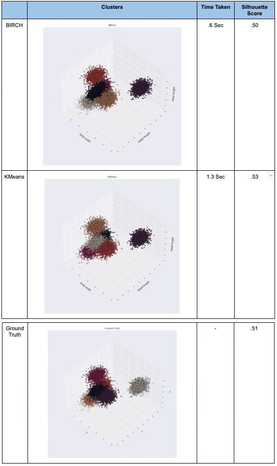
        return t1-t0

We will now compare silhouette score for both the approaches. Silhouette scores will suggest how well-separated clusters are. Comparing this with original cluster labelling (ground truth) will give us a good idea as to which approach is providing more similar results to ground truth.

This will be followed by visually inspecting the results using 3D scatter diagram of clusters.

###################### silhouette score #################
def get_silhouette_score(df,algo,clusters):
    if algo == 'KMeans':
        kmeans = KMeans(n_clusters=clusters,
                        random_state=10)
        kmeans.fit(df)
        labels = kmeans.labels_        return metrics.silhouette_score(df, labels)
        
    elif algo == 'BIRCH':
        brc = Birch(branching_factor=50, 
                    n_clusters=clusters, 
                    threshold=1)
        brc.fit(df)
        labels = brc.labels_        return metrics.silhouette_score(df, labels)################# Visualizing K-Means Vs BIRCH results #######
estimators = [
    ("k_means", KMeans(n_clusters=6,
                              random_state=10)),
    ("BIRCH", Birch(branching_factor=50, 
                    n_clusters=6, 
                    threshold=.5)),
]fignum = 1
titles = ["KMeans", "BIRCH"]
for name, est in estimators:
    fig = plt.figure(fignum, figsize=(10, 15))
    ax = Axes3D(fig, rect=[0, 0, 0.95, 1], elev=48, azim=134)
    est.fit(X)
    labels = est.labels_    ax.scatter(X[:, 1], X[:, 0], X[:, 2], c=labels.astype(float),     edgecolor="k")
    ax.set_xlabel("X")
    ax.set_ylabel("Y")
    ax.set_zlabel("Z")
    ax.set_title(titles[fignum - 1])
    ax.dist = 12
    fignum = fignum + 1# Plot the ground truth
fig = plt.figure(fignum, figsize=(10, 15))
ax = Axes3D(fig, rect=[0, 0, 0.95, 1], elev=48, azim=134)ax.scatter(X[:, 1], X[:, 0], X[:, 2], c=clusters, edgecolor="k")ax.set_xlabel("X")
ax.set_ylabel("Y")
ax.set_zlabel("Z")
ax.set_title("Ground Truth")
ax.dist = 12fig.show()

(a) Time taken/silhouette scores may vary slightly in each run

Conclusion

From the results above, we can make the following inferences on BIRCH for the given dataset.

1. Visually, K-Means and BIRCH provide quite similar results.
2. There is a significant improvement in time elapsed (~50%) over K-Means. With hyper-parameter tuning this might improve further.
3. Silhouette score is very similar for all three KMeans ,BIRCH and ground truth implying BIRCH is not compromising on the cluster quality. One might think of a reduction in silhouette score in BIRCH due to its inherent methodology of summarizing data before performing clustering.

You can access notebook at: https://www.kaggle.com/code/blackburn1/birch-implementation-and-comparision-with-kmeans?scriptVersionId=91993527

You can also check out other articles written around data science, computing on medium. If you like my work and want to contribute to my journey, you cal always buy me a coffee :)

References

[1] Original Paper: https://www2.cs.sfu.ca/CourseCentral/459/han/papers/zhang96.pdf

[2] Sklearn: https://scikit-learn.org/stable/modules/clustering.html#birch

[3] Explanation on BIRCH phases: https://towardsdatascience.com/machine-learning-birch-clustering-algorithm-clearly-explained-fb9838cbeed9

[4] K-Means Clustering example: https://scikit-learn.org/stable/auto_examples/cluster/plot_cluster_iris.html#sphx-glr-auto-examples-cluster-plot-cluster-iris-py

[5] Silhouette score: https://scikit-learn.org/stable/modules/generated/sklearn.metrics.silhouette_score.html