Step-by-Step Guide Towards Time Series Forecasting
We will take a problem of forecasting hourly passenger demands based on the historical data and follow a set of steps to perform forecasting. Framework learnt here could be smoothly applied to any general time series forecasting problem.
Introduction
Approaching a timeseries problem is usually not very straightforward as there could be multiple ways to approach a certain problem. Specially, once you are done with basic EDA, and want to proceed with application of forecasting models.
In this Article, our goal is to learn how to systematically approach forecasting problem. Framework can be replicated in other problems with some tweaks.
It is to be noted that systematic approach might not lead to the most optimal solution. However, it would definitely lead to a reasonably good solution which can be enhanced after more experimentation depending on the complexity of the problem.
Problem statement
In this problem, we are given a time series data of train passensers for last three years on an hourly basis and our goal is to forecast future demands. Below is how the data looks:
https://gist.github.com/girish9851/6b27412b29df8b5b057f7f4801bf5415#file-table_head_2-csv
We have just hourly timestamp and count other than ID. we are supposed to forecast Count for future dates basis the train data.
Lets proceed with exploring dataset.
Data exploration
Hourly Time-series from of demand

We can see some seasonality in data and a clear increasing trend in the demand.
To make our forecasting process relatively easier, lets try to forecast daily demand and distribute that based on the avarge hourly distribution of a day on the basis of hisotrical data.
Daily Time-series data of demand

After daily grouping, data is more readable and would be rather easier to analyse and forecast.
Below is the hourly distribution on an average. To make our forecasting even more nuanced, Its possible to have a better approach to forecast hourly split but for now we will continue with average numbers.

Stationarity and other properties of time series
A very straight forward approach to study trend, seasonality is time series decomposition. In this approach, we assign a reasonable estimate of seasonality and then remove the trend and residual part from the original timeries as depicted in the chart below:

As we can see that variability of residuals is not constant and its increasing in a quadratic manner , suggesting that variability of the time-series is increasing. An approach to handle such situations by applying
transformations such as log transformation or square root transformation. Below is once we transform the data by applying log transformations — we can clearly see the change in variability of residuals and they do not show Heteroskedasticity any more:
Lets now look at the Auto correlation function plot and partial auto correlation function plot to represent the relationships among the lagged variables. Below are the results in a data with no transformation applied:


We can see that there is a weekly seasonality as every 7th PACF value is significant and similarly we have ACF show a distinct wavy structure to indicate seasonality.
Now lets try to make similar observations with square root transformed data:


Observations : we see that ACF is decaying with lags and PACF abruptly becomes insignificant after some lags. This combination suggests that the time series have both AR and MA components.
We also observe some kind of seasonality in the PACF and ACF which seems to be weekly. Hence it can be concluded that the time series has seasonlity effect as well.
Forecasting
we will start exploring in the following order:
(1) AR
(2) MA
(3) AR with differencing
(4) MA with differencing
(5) ARMA
(6) ARIMA (ARMA with differencing)
(7) SARIMA (initial model)
(8) SARIMA (after hyperparameter tuning of p,q,d,P,Q,D,s )
- AR (7) without differencing
# Importing necessary libraries
import statsmodels.api as sm
import matplotlib.pyplot as plt

# Creating a SARIMAX model with AR (7) order
mod = sm.tsa.statespace.SARIMAX((df.Count),
                                order=(7,0,0),
                                seasonal_order=(0,0,0,0))

# Fitting the model and obtaining the results
results = mod.fit()

# Predicting values for the test set dynamically from a specific starting point to an ending point
a_preds_AR = results.predict(start=762, end=974, dynamic=True)

# Predicting values for the training set from the beginning up to a specific point without dynamic updating
preds_old_AR = results.predict(start=0, end=761, dynamic=False)

# Plotting the predicted values for the test and training sets
plt.plot(a_preds_AR, label='test')
plt.plot(preds_old_AR, label='train')

# Adding legend, xlabel, ylabel, and title to the plot
plt.legend('upperleft')
plt.xlabel('date')
plt.ylabel('Count')
plt.title('AR(7) with no seasonality effect')
2. MA (7) without differencing
# Importing necessary libraries
import statsmodels.api as sm
import matplotlib.pyplot as plt

# Creating a SARIMAX model with specified order and seasonal order for
# moving average (MA) with order 7
mod = sm.tsa.statespace.SARIMAX((df.Count),
                                order=(0,0,7),
                                seasonal_order=(0,0,0,0))

# Fitting the model and obtaining the results
results = mod.fit()

# Predicting values for the test set dynamically from a specific starting point to an ending point
a_preds_MA = results.predict(start=762, end=974, dynamic=True)

# Predicting values for the training set from the beginning up to a specific point without dynamic updating
preds_old_MA = results.predict(start=0, end=761, dynamic=False)

# Plotting the predicted values for the test and training sets
plt.plot(a_preds_MA, label='test')
plt.plot(preds_old_MA, label='train')

# Adding legend, xlabel, ylabel, and title to the plot
plt.legend('upperleft')
plt.xlabel('date')
plt.ylabel('Count')
plt.title('MA(7) with no seasonality effect')
3. AR (7) with differencing
# Importing necessary libraries
import statsmodels.api as sm
import matplotlib.pyplot as plt

# Creating a SARIMAX model with specified order and seasonal
# order for autoregressive (AR) with order 7 and first-order differencing
mod = sm.tsa.statespace.SARIMAX((df.Count),
                                 order=(7,1,0),
                                 seasonal_order=(0,0,0,0))

# Fitting the model and obtaining the results
results = mod.fit()

# Predicting differenced values for the test set dynamically from a specific starting point to an ending point
a_preds_AR_diff = results.predict(start=762, end=974, dynamic=True)

# Predicting differenced values for the training set from the beginning up to a specific point without dynamic updating
preds_old_AR_diff = results.predict(start=0, end=761, dynamic=False)

# Plotting the predicted differenced values for the test and training sets
plt.plot(a_preds_AR_diff, label='test')
plt.plot(preds_old_AR_diff, label='train')

# Adding legend, xlabel, ylabel, and title to the plot
plt.legend('upperleft')
plt.xlabel('date')
plt.ylabel('Count')
plt.title('AR(7) with differencing with no seasonality effect')
4. MA (7) with differencing
# Importing necessary libraries
import statsmodels.api as sm
import matplotlib.pyplot as plt

# Creating a SARIMAX model with specified order and seasonal order
# for moving average (MA) with order 7 and first-order differencing
mod = sm.tsa.statespace.SARIMAX((df.Count), order=(0,1,7), seasonal_order=(0,0,0,0))

# Fitting the model and obtaining the results
results = mod.fit()

# Predicting differenced values for the test set dynamically from a specific starting point to an ending point
a_preds_MA = results.predict(start=762, end=974, dynamic=True)

# Predicting differenced values for the training set from the beginning up to a specific point without dynamic updating
preds_old_MA = results.predict(start=0, end=761, dynamic=False)

# Plotting the predicted differenced values for the test and training sets
plt.plot(a_preds_MA, label='test')
plt.plot(preds_old_MA, label='train')

# Adding legend, xlabel, ylabel, and title to the plot
plt.legend('upperleft')
plt.xlabel('date')
plt.ylabel('Count')
plt.title('MA(7) with differencing and no seasonality effect')
5. ARMA without diff and no seasonality
# Importing necessary libraries
import statsmodels.api as sm
import matplotlib.pyplot as plt

# Creating a SARIMAX model with specified order and seasonal order
# for autoregressive moving average (ARMA) with order 7 and no differencing
mod = sm.tsa.statespace.SARIMAX((df.Count), order=(7,0,7), seasonal_order=(0,0,0,0))

# Fitting the model and obtaining the results
results = mod.fit()

# Predicting values for the test set dynamically from a specific starting point to an ending point
a_preds_ARMA = results.predict(start=762, end=974, dynamic=True)

# Predicting values for the training set from the beginning up to a specific point without dynamic updating
preds_old_ARMA = results.predict(start=0, end=761, dynamic=False)

# Plotting the predicted values for the test and training sets
plt.plot(a_preds_ARMA, label='test')
plt.plot(preds_old_ARMA, label='train')

# Adding legend, xlabel, ylabel, and title to the plot
plt.legend('upperleft')
plt.xlabel('date')
plt.ylabel('Count')
plt.title('ARMA(7,7) with differencing with no seasonality effect')
6. ARIMA with 1 differencing p= 7, d= 1, q = 7
# Importing necessary libraries
import statsmodels.api as sm
import matplotlib.pyplot as plt

# Creating a SARIMAX model with specified order and seasonal order for autoregressive integrated moving average (ARIMA) with order (7,1,7)
mod = sm.tsa.statespace.SARIMAX((df.Count), order=(7,1,7), seasonal_order=(0,0,0,0))

# Fitting the model and obtaining the results
results = mod.fit()

# Predicting differenced values for the test set dynamically from a specific starting point to an ending point
a_preds_ARIMA = results.predict(start=762, end=974, dynamic=True)

# Predicting differenced values for the training set from the beginning up to a specific point without dynamic updating
preds_old_ARIMA = results.predict(start=0, end=761, dynamic=False)

# Plotting the predicted differenced values for the test and training sets
plt.plot(a_preds_ARIMA, label='test')
plt.plot(preds_old_ARIMA, label='train')

# Adding legend, xlabel, ylabel, and title to the plot
plt.legend('upperleft')
plt.xlabel('date')
plt.ylabel('Count')
plt.title('ARIMA(7,1,7) with differencing with no seasonality effect')
7. SARIMA with order (p=1,d=1,q=1) & (P=1, D=0, Q=1, S=7)
Now let’s explicitly consider seasonality part with ARIMA model. We now need to decrease the order of ARIMA model between 1–6 (both AR, MA) as it should not be same as season order (we would not be able to capture effects properly if we perform either MA/AR on the same order as seasonility.
Lets also take seasonal seasonal AR and MA orders of 1 as our intent is also to capture any auto regression or moving average characteristic in the seasonality.
# Importing necessary libraries
import statsmodels.api as sm
import matplotlib.pyplot as plt

# Creating a SARIMAX model with specified order and seasonal order for seasonal autoregressive integrated moving average (SARIMA)
# with order (1,1,1) and seasonal order (1,0,1,7)
mod = sm.tsa.statespace.SARIMAX((df.Count),
                                  order=(1,1,1),
                                  seasonal_order=(1,0,1,7))

# Fitting the model and obtaining the results
results = mod.fit()

# Predicting values for the test set dynamically from a specific starting point to an ending point
a_preds_SARIMA = results.predict(start=762, end=974, dynamic=True)

# Predicting values for the training set from the beginning up to a specific point without dynamic updating
preds_old_SARIMA = results.predict(start=0, end=761, dynamic=False)

# Plotting the predicted values for the test and training sets
plt.plot(a_preds_SARIMA, label='test')
plt.plot(preds_old_SARIMA, label='train')

# Adding legend, xlabel, ylabel, and title to the plot
plt.legend('upperleft')
plt.xlabel('date')
plt.ylabel('Count')
plt.title('SARIMA(1,1,1),(1,0,1,7)')
plt.show()
8. SARIMA with (p=1,d=1,q=1) & (P=1, D=1, Q=0, S=7) on sqrt tranformed data
# Importing necessary libraries
import statsmodels.api as sm
import matplotlib.pyplot as plt
import numpy as np

# Applying square root transformation to the 'Count' values
transformed_count = np.sqrt(df.Count)

# Creating a SARIMAX model with specified order and seasonal order
# for seasonal autoregressive integrated moving average (SARIMA)
# with order (1,1,1) and seasonal order (1,0,1,7) on the
# transformed 'Count' values
mod = sm.tsa.statespace.SARIMAX(transformed_count, order=(1,1,1), seasonal_order=(1,0,1,7))

# Fitting the model and obtaining the results
results = mod.fit()

# Predicting transformed values for the test set dynamically
#from a specific starting point to an ending point
a_preds_SARIMA = results.predict(start=762, end=974, dynamic=True)

# Predicting transformed values for the training set from
# the beginning up to a specific point without dynamic updating
preds_old_SARIMA = results.predict(start=0, end=761, dynamic=False)

# Applying inverse transformation (square) to get predictions
# in the original scale
a_preds_SARIMA_original = np.square(a_preds_SARIMA)
preds_old_SARIMA_original = np.square(preds_old_SARIMA)

# Plotting the predicted values for the test and training sets in the original scale
plt.plot(a_preds_SARIMA_original, label='test')
plt.plot(preds_old_SARIMA_original, label='train')

# Adding legend, xlabel, ylabel, and title to the plot
plt.legend('upperleft')
plt.xlabel('date')
plt.ylabel('Count')
plt.title('SARIMA(1,1,1),(1,0,1,7) with sqrt transformation')
plt.show()
9. SARIMA with (p=1,d=1,q=1) & (P=1, D=0, Q=1, S=7) on log transformed data
Lets try same approach as above two SARIMA models but on log transformed data.
# Importing necessary libraries
import statsmodels.api as sm
import matplotlib.pyplot as plt
import numpy as np

# Applying natural logarithm transformation to the 'Count' values
log_transformed_count = np.log(df.Count)

# Creating a SARIMAX model with specified order and seasonal order for
# seasonal autoregressive integrated moving average (SARIMA)
# with order (1,1,1) and seasonal order (1,0,1,7) on the
# log-transformed 'Count' values
mod = sm.tsa.statespace.SARIMAX(log_transformed_count, order=(1,1,1), seasonal_order=(1,0,1,7))

# Fitting the model and obtaining the results
results = mod.fit()

# Predicting transformed values for the test set dynamically
# from a specific starting point to an ending point
a_preds_SARIMA = results.predict(start=762, end=974, dynamic=True)

# Predicting transformed values for the training set from the
# beginning up to a specific point without dynamic updating
preds_old_SARIMA = results.predict(start=0, end=761, dynamic=False)

# Applying inverse transformation (exponential) to get predictions
# in the original scale
a_preds_SARIMA_original = np.exp(a_preds_SARIMA)
preds_old_SARIMA_original = np.exp(preds_old_SARIMA)

# Plotting the predicted values for the test and training sets
# in the original scale
plt.plot(a_preds_SARIMA_original, label='test')
plt.plot(preds_old_SARIMA_original, label='train')

# Adding legend, xlabel, ylabel, and title to the plot
plt.legend('upperleft')
plt.xlabel('date')
plt.ylabel('Count')
plt.title('SARIMA(1,1,1),(1,0,1,7)')
plt.show()
10. Using pmdarima for hyper-parameter tuning and model selection
Now we can use metrics like AIC to optimise the order — for this we would use auto_arima from pmdarima module. below snippent shows the flow for applying auto_arima on log transformed data:
# Importing necessary libraries
import pmdarima as pm
import statsmodels.api as sm
import matplotlib.pyplot as plt
import numpy as np

# Performing automatic ARIMA model selection using pmdarima
model = pm.auto_arima(np.log(df.Count), start_p=1, start_q=1,
                      test='adf',
                      max_p=6, max_q=6, m=7,
                      start_P=0, seasonal=True,
                      d=1, D=1, trace=True, stationary=False,
                      error_action='ignore',
                      suppress_warnings=True, with_intercept=False,
                      stepwise=True)

# Creating a SARIMAX model with the selected hyperparameters
# from the auto_arima model selection
mod = sm.tsa.statespace.SARIMAX(np.log(df.Count), order=model.order, seasonal_order=model.seasonal_order)

# Fitting the model and obtaining the results
results = mod.fit()

# Predicting transformed values for the test set dynamically
# from a specific starting point to an ending point
a_preds_SARIMA_log_tuned = results.predict(start=762, end=974, dynamic=True)

# Predicting transformed values for the training set from
# the beginning up to a specific point without dynamic updating
preds_old_SARIMA_log_tuned = results.predict(start=0, end=761, dynamic=False)

# Applying inverse transformation (exponential) to get
# predictions in the original scale
a_preds_SARIMA_tuned = np.exp(a_preds_SARIMA_log_tuned)
preds_old_SARIMA_tuned = np.exp(preds_old_SARIMA_log_tuned)

# Plotting the predicted values for the test and training sets
# in the original scale
plt.plot(a_preds_SARIMA_tuned, label='test')
plt.plot(preds_old_SARIMA_tuned, label='train')

# Adding legend, xlabel, ylabel, and title to the plot
plt.legend('upperleft')
plt.xlabel('date')
plt.ylabel('Count')
plt.title('SARIMA with hyperparameter tuning # SARIMAX {} x {}'.format(model.order,model.seasonal_order))
plt.show()
Lets see results on all three variants — no transformation, square root transformation and log tranformation:
10.1 no transformation

10.2 sqrt transformed data

10.3 log transformed data sarima optimisation

Although it’s difficult to visually decipher if auto arima has really improved the results or not, AIC is indeed optimised so we could reasonably believe that test results would be better than any of the models above
Converting model selection results on daily data to hourly
Let’s now use the daily prediction results from log transformed data and convert that to hourly using the mean hourly distribution calculated above.
# Converting sum2 to a list
listm = list(sum2)
# Exponentiating the predicted SARIMA values to obtain predictions in the original scale
prediction = np.exp(a_preds_SARIMA_log_tuned)
# Initializing an empty list to store errors
er = []
# Iterating through the predictions and listm to calculate hourly numbers
for p in range(len(prediction)):
for l in range(len(listm)):
er.append(prediction[p] * listm[l])
# Creating a DataFrame with the calculated hourly numbers
d = {'Count': er}
predflog = pd.DataFrame(data=d)
# Reading the test data for submission
sublog = pd.read_csv('./input/Test.csv')
# Updating the 'Count' column in the submission data with the predicted values
sublog['Count'] = predflog['Count']
# Saving the updated submission data to a CSV file
sublog.to_csv("submlog.csv", index=False)
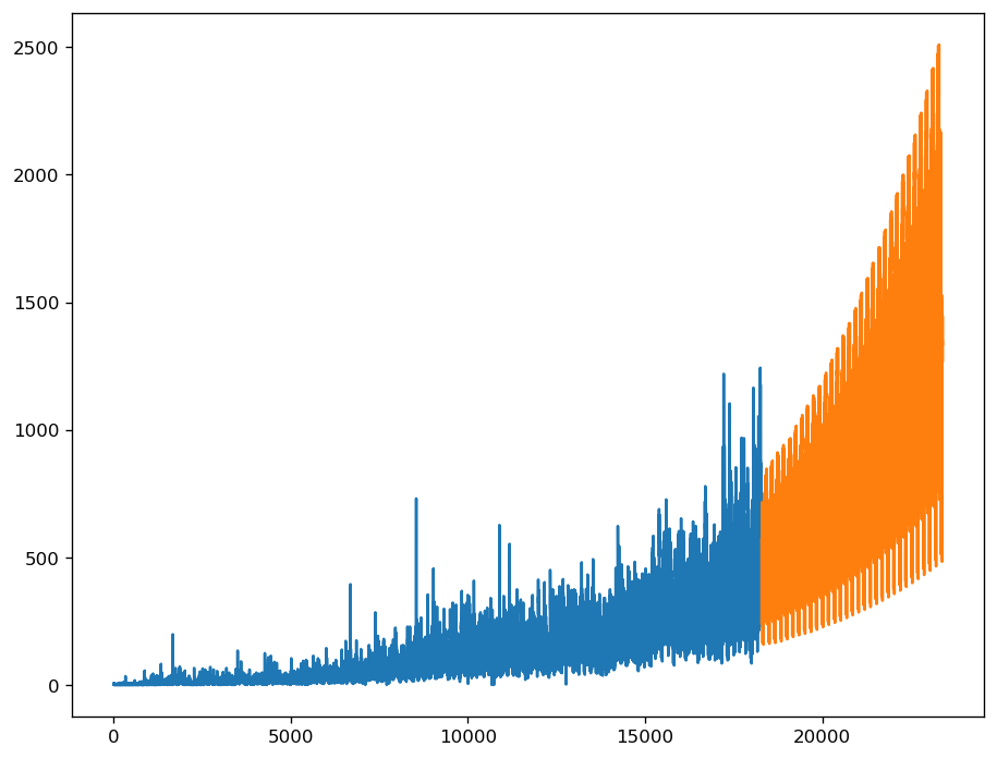
# Plotting the original 'Count' from df1 and the predicted 'Count' from the submission data
plt.plot(df1['Count'])
plt.plot(sublog['ID'], sublog['Count'])
Ensemble model — 1
# Calculating the ensemble prediction by averaging SARIMA predictions in different scales
ensembled_prediction = (a_preds_SARIMA_tuned + np.exp(a_preds_SARIMA_log_tuned) + np.square(a_preds_SARIMA_sqrt_tuned)) / 3

# Plotting the ensembled predictions for the test set and the predictions for the training set
plt.plot(ensembled_prediction, label='test')
plt.plot(preds_old_SARIMA_tuned, label='train')

# Adding legend, xlabel, ylabel, and title to the plot
plt.legend('upperleft')
plt.xlabel('date')
plt.ylabel('Count')
plt.title('SARIMA with hyperparameter tuning # ensemble')
plt.show()
Ensemble model — 2
Now a rather complicated ensemble of:
- SARIMA on log transformed data
- SARIMA on log transformed data detrended + SARIMA on (seasonality + residuals)
Lets start with detrending the log transformed data

Lets now apply model selection on detrended and trend data and add them together to get the results
# Importing necessary libraries
from statsmodels.tsa.seasonal import seasonal_decompose
import pmdarima as pm
import statsmodels.api as sm
import matplotlib.pyplot as plt
import numpy as np
import pandas as pd

# Performing seasonal decomposition of the log-transformed 'Count'
# using additive model with a period of 7
result = seasonal_decompose(np.log(df.Count), model='additive', period=7)

# Obtaining detrended data by adding seasonal and residual components,
# and trend data
detrended_Data = (result.seasonal + result.resid).dropna()
trend_Data = result.trend.dropna()

# Performing automatic ARIMA model selection on the detrended data
# using pmdarima
model = pm.auto_arima(detrended_Data, start_p=1, start_q=1,
                      test='adf',
                      max_p=6, max_q=6, m=7,
                      start_P=0, seasonal=True,
                      d=1, D=1, trace=True, stationary=False,
                      error_action='ignore',
                      suppress_warnings=True, with_intercept=False,
                      stepwise=True)

# Creating a SARIMAX model with the selected hyperparameters from
# the auto_arima model selection for detrended data
mod = sm.tsa.statespace.SARIMAX(detrended_Data, order=model.order, seasonal_order=model.seasonal_order)
results = mod.fit()

# Predicting detrended values using the SARIMAX model
a_preds_SARIMA_log_tunedm = results.predict(start=759, end=971, dynamic=True)
preds_old_SARIMA_log_tunedm = results.predict(start=0, end=759, dynamic=False)

# Creating a SARIMAX model for trend data
mod = sm.tsa.statespace.SARIMAX(trend_Data, order=(1,1,0), seasonal_order=(0,1,1,30))
results = mod.fit()
print(results.summary())  # Printing the summary of the model results

# Predicting trend values using the SARIMAX model
a_preds_SARIMA_log_tunedmt = results.predict(start=759, end=971, dynamic=True)
preds_old_SARIMA_log_tunedmt = results.predict(start=0, end=759, dynamic=False)

# Plotting the ensemble predictions for the test set and the predictions
# for the training set
plt.plot(np.exp(a_preds_SARIMA_log_tunedm + a_preds_SARIMA_log_tunedmt), label='test')
plt.plot(np.exp(preds_old_SARIMA_log_tunedm + preds_old_SARIMA_log_tunedmt), label='train')
plt.legend('upperleft')
plt.xlabel('date')
plt.ylabel('Count')
plt.title('SARIMA with hyperparameter tuning detrended - (6, 1, 0)x(0, 1, [2], 7) & trend - (1,1,0)x(0,1,1,30)')
plt.show()

# Calculating the ensemble prediction by averaging predictions from
# SARIMA models in different scales
ensembled_prediction1 = (np.exp(a_preds_SARIMA_log_tunedm + a_preds_SARIMA_log_tunedmt) +
                         np.exp(a_preds_SARIMA_log_tuned)) / 2

# Plotting the ensemble predictions for the test set and the predictions
# for the training set
plt.plot(ensembled_prediction1, label='test')
plt.plot(np.exp(preds_old_SARIMA_log_tuned), label='train')
plt.legend('upperleft')
plt.xlabel('date')
plt.ylabel('Count')
plt.title('SARIMA with hyperparameter tuning # ensemble')
plt.show()

# Creating a DataFrame with the calculated ensemble predictions multiplied
# by 'listm'
listm = list(sum2)
er = []

for p in range(len(ensembled_prediction1)):
    for l in range(len(listm)):
        er.append(ensembled_prediction1[p] * listm[l])

d = {'Count': er}
predf = pd.DataFrame(data=d)

# Reading the test data for submission
sub = pd.read_csv('./input/Test.csv')

# Updating the 'Count' column in the submission data with the predicted
# values
sub['Count'] = predf['Count']

# Saving the updated submission data to a CSV file
sub.to_csv("subm.csv", index=False)

# Plotting the original 'Count' from df1 and the predicted 'Count' from
# the submission data
plt.plot(df1['Count'])
plt.plot(sub['ID'], sub['Count'])


Accuracy measurement
Since this problem was a part of an analytics vidya competition, we have test RMSE scores only and not the actual test data
Below are the results:
Ensemble- 1 of SARIMA on log transformed data — RMSE: 146
Ensemble- 2 of SARIMA on log transformed data + SARIMA on detrended and trend splits of log transformed data — RMSE: 144
We have also kept a track of AIC values for various models used above while performing model selection using pmdarima module.
Further improvements
One of the key drawbacks here is that we are considering average of hourly distribution which is not the best way. One possible way is to apply forecasting on daily distribution.
References
- Github link to notebook — https://github.com/girish9851/Time-Series-Practice-problem-AV/blob/master/Final_code.ipynb
- Analytics Vidhya — https://datahack.analyticsvidhya.com/contest/practice-problem-time-series-2/
If you found the explanation helpful, follow me for more content! Feel free to leave comments with any questions or suggestions you might have.
You can also check out other articles written around data science, computing on medium. If you like my work and want to contribute to my journey, you cal always buy me a coffee :)


Comments
Post a Comment